Accelerometer sensor
- An electromechanical device used to measure acceleration forces.
- Such forces may be static, like the continuous force of gravity
- As is the case with many mobile devices – dynamic to sense movement or walking.
- Two types (a) the piezoelectric effect and (2) the capacitance sensor.
- Most smartphones typically make use of three-axis models to determine the moment of impact
- The sensitivity of these devices is quite high as they’re intended to measure even very minute shifts in acceleration. The more sensitive the accelerometer, the more easily it can measure acceleration.
- Internal circuitry converts the tiny capacitance to a voltage signal which is digitized and output
- Computing orientation from an accelerometer relies on a constant gravitational pull of 1g (9.8 m/s^2) downwards
- If no additional forces act on the accelerometer (a risky assumption), the magnitude of the acceleration is 1g, and the sensor’s rotation can be computed from the position of the acceleration vector
- If the Z-axis is aligned along the gravitational acceleration vector, it is impossible to compute rotation around the Z-axis from the accelerometer.
- Digital accelerometers give information using a serial protocol like I2C , SPI or USART; analog accelerometers output a voltage level within a predefined range.
- Each accelerometer has a zero-g voltage level, you can find it in spec
- Accelerometers also have a sensitivity, usually expressed in mV/g
- Divide the zero-g level corrected reading by the sensitivity to produce the final reading

When thinking about accelerometers it is often useful to image a box in shape of a cube with a ball inside it. You may imagine something else like a cookie or a donut , but I’ll imagine a ball:

If we take this box in a place with no gravitation fields or for that matter with no other fields that might affect the ball’s position – the ball will simply float in the middle of the box. You can imagine the box is in outer-space far-far away from any cosmic bodies, or if such a place is hard to find imagine at least a space craft orbiting around the planet where everything is in weightless state . From the picture above you can see that we assign to each axis a pair of walls (we removed the wall Y+ so we can look inside the box). Imagine that each wall is pressure sensitive. If we move suddenly the box to the left (we accelerate it with acceleration 1g = 9.8m/s^2), the ball will hit the wall X-. We then measure the pressure force that the ball applies to the wall and output a value of -1g on the X axis.

Please note that the accelerometer will actually detect a force that is directed in the opposite direction from the acceleration vector. This force is often called Inertial Force or Fictitious Force . One thing you should learn from this is that an accelerometer measures acceleration indirectly through a force that is applied to one of it’s walls (according to our model, it might be a spring or something else in real life accelerometers). This force can be caused by the acceleration , but as we’ll see in the next example it is not always caused by acceleration.
If we take our model and put it on Earth the ball will fall on the Z- wall and will apply a force of 1g on the bottom wall, as shown in the picture below:

In this case the box isn’t moving but we still get a reading of -1g on the Z axis. The pressure that the ball has applied on the wall was caused by a gravitation force. In theory it could be a different type of force – for example, if you imagine that our ball is metallic, placing a magnet next to the box could move the ball so it hits another wall. This was said just to prove that in essence accelerometer measures force not acceleration. It just happens that acceleration causes an inertial force that is captured by the force detection mechanism of the accelerometer.
While this model is not exactly how a MEMS sensor is constructed it is often useful in solving accelerometer related problems. There are actually similar sensors that have metallic balls inside, they are called tilt switches, however they are more primitive and usually they can only tell if the device is inclined within some range or not, not the extent of inclination.
So far we have analyzed the accelerometer output on a single axis and this is all you’ll get with a single axis accelerometers. The real value of triaxial accelerometers comes from the fact that they can detect inertial forces on all three axes. Let’s go back to our box model, and let’s rotate the box 45 degrees to the right. The ball will touch 2 walls now: Z- and X- as shown in the picture below:
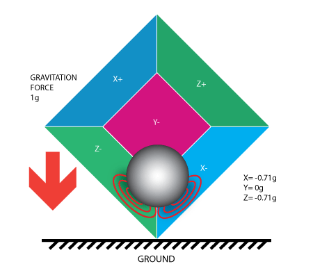
The values of 0.71 are not arbitrary, they are actually an approximation for SQRT(1/2). This will become more clear as we introduce our next model for the accelerometer.
Estimating the Inclination Angle with an Accelerometer
As mentioned above, we would need to get a good measurement of the current inclination angle in order to control the robot’s movements. Let’s first examine how to use an accelerometer alone to measure the inclination angle.
Suppose that the robot is a stationary position illustrated below (viewed from the side, accelerometer is placed on the top of the robot, perpendicular to the body):
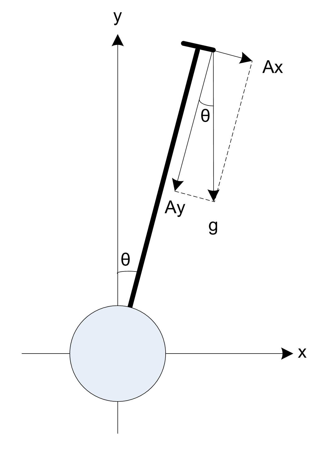
The inclination angle can be calculated as:
cos(Axr) = Rx / R
cos(Ayr) = Ry / R
cos(Azr) = Rz / R
R = SQRT( Rx^2 + Ry^2 + Rz^2)
Find angles by using arccos() function (the inverse cos() function ):
Axr = arccos(Rx/R)
Ayr = arccos(Ry/R)
Azr = arccos(Rz/R)
A typical accelerometer has the following basic specifications:
-
Analog/digital
-
Number of axes
-
Output range (maximum swing)
-
Sensitivity (voltage output per g)
-
Dynamic range
-
Bandwidth
-
Amplitude stability
-
Mass
Analog vs. digital: The most important specification of an accelerometer for a given application is its type of output.
Analog accelerometers output a constant variable voltage depending on the amount of acceleration applied. Older digital accelerometers output a variable frequency square wave, a method known as pulse-width modulation. A pulse width modulated accelerometer takes readings at a fixed rate, typically 1000 Hz (though this may be user-configurable based on the IC selected). The value of the acceleration is proportional to the pulse width (or duty cycle) of the PWM signal.
Newer digital accelerometers (MPU6050, MPU9250) are more likely to output their value using multi-wire digital protocols such as I2C or SPI. For use with accelerometers commonly used for healthcare monitoring, pedometer, gait analysis systems.
Number of axes: Accelerometers are available that measure in one, two, or three dimensions. The most familiar three-axis accelerometers are increasingly common and inexpensive.
Output range: To measure the acceleration of gravity for use as a tilt sensor, an output range of ±1 g, ±2 g, ±3 g, ±4 g available.
Sensitivity: An indicator of the amount of change in output signal for a given change in acceleration. A sensitive accelerometer will be more precise and probably more accurate.
Dynamic range: The range between the smallest acceleration detectable by the accelerometer to the largest before distorting or clipping the output signal.
Bandwidth: The bandwidth of a sensor is usually measured in Hertz and indicates the limit of the near-unity frequency response of the sensor, or how often a reliable reading can be taken. Humans cannot create body motion much beyond the range of 10-12 Hz. For this reason, a bandwidth of 40-60 Hz is adequate for tilt or human motion sensing. For vibration measurement or accurate reading of impact forces, bandwidth should be in the range of hundreds of Hertz. It should also be noted that for some older microcontrollers, the bandwidth of an accelerometer may extend beyond the Nyquist frequency of the A/D converters on the MCU, so for higher bandwidth sensing, the digital signal may be aliased. This can be remedied with simple passive low-pass filtering prior to sampling, or by simply choosing a better microcontroller. It is worth noting that the bandwidth may change by the way the accelerometer is mounted. A stiffer mounting (ex: using studs) will help to keep a higher usable frequency range and the opposite (ex: using a magnet) will reduce it.
Amplitude stability: This is not a specification in itself, but a description of several. Amplitude stability describes a sensor’s change in sensitivity depending on its application, for instance over varying temperature or time (see below).
Mass: The mass of the accelerometer should be significantly smaller than the mass of the system to be monitored so that it does not change the characteristic of the object being tested.
Tolerance: It’s the maximum error of frequency response. The parameter error of 32 kΩ ± 15%.
Other specifications include:
-
Zero g offset (voltage output at 0 g)
-
Noise (sensor minimum resolution)
-
Temperature range
-
Bias drift with temperature (effect of temperature on voltage output at 0 g)
-
Sensitivity drift with temperature (effect of temperature on voltage output per g)
-
Power consumption
Output
An accelerometer output value is a scalar corresponding to the magnitude of the acceleration vector. The most common acceleration, and one that we are constantly exposed to, is the acceleration that is a result of the earth’s gravitational pull. This is a common reference value from which all other accelerations are measured (known as g, which is ~9.8m/s^2).
Digital output
Accelerometers with PWM output can be used in two different ways. For most accurate results, the PWM signal can be input directly to a microcontroller where the duty cycle is read in firmware and translated into a scaled acceleration value. (Check with the datasheet to obtain the scaling factor and required output impedance.) When a microcontroller with PWM input is not available, or when other means of digitizing the signal are being used, a simple RC reconstruction filter can be used to obtain an analog voltage proportional to the acceleration. At rest (50% duty-cycle) the output voltage will represent no acceleration, higher voltage values (resulting from a higher duty cycle) will represent positive acceleration, and lower values (<50% duty cycle) indicate negative acceleration. These voltages can then be scaled and used as one might the output voltage of an analog output accelerometer. One disadvantage of a digital output is that it takes a little more timing resources of the microcontroller to measure the duty cycle of the PWM signal. Communication protocols could use I2C or SPI.
Analog output
When compared to most other industrial sensors, analog accelerometers require little conditioning and the communication is simple by only using an Analog to Digital Converter (ADC) on the microcontroller. Typically, an accelerometer output signal will need an offset, amplification, and filtration. For analog voltage output accelerometers, the signal can be a positive or negative voltage, depending on the direction of the acceleration. Also, the signal is continuous and proportional to the acceleration force. As with any sensor destined for an analog to digital converter, the value must be scaled and/or amplified to maximally span the range of acquisition. Most analog to digital converters used in musical applications acquire signals in the 0-5 V range.
The image at right depicts an amplification and offset circuit, including the on-board operational amplifier in the adxl 105, minimizing the need for additional IC components. The gain applied to the output is set by the ratio R2/R1. The offset is controlled by biasing the voltage with variable resistor R4. Accelerometers output bias will drift according to ambient temperature. The sensors are calibrated for operation at a specific temperature, typically room temperature. However, in most short duration indoor applications the offset is relatively constant and stable, and thus does not need adjustment. If the sensor is intended to be used in multiple environments with differing ambient temperatures, the bias function should be sufficient for analog calibration of the device. If the ambient temperature is subject to drastic changes over the course of a single usage, the temperature output should be summed into the bias circuit. Smart sensors may even take this into consideration.
The resolution of the data acquired is ultimately determined by the analog to digital converter. It is possible, however, that the noise floor is above the minimum resolution of the converter, reducing the resolution of your system. Assuming that the noise is equally distributed across all frequencies, it is possible to filter the signal to only include frequencies within the range of operation. The filter required depends upon both the type of acquisition as well as the location of the sensor. The bandwidth is primarily influenced by the three different modes of operation of the sensor.
Ref. Study link
- Here, a good article how to apply complimentary filter algorithm to a balancing robot: http://www.kerrywong.com/2012/03/08/a-self-balancing-robot-i/
-
MPU6050
https://www.invensense.com/products/motion-tracking/6-axis/mpu-6050/
- [I2C Prptocol]


14/07/2016 at 3:54 pm
http://projectallyy.blogspot.in/2015/10/3d-visualization-display.html
14/07/2016 at 4:16 pm
[2] Here, a good article how to apply complimentary filter algorithm to a balancing robot: http://www.kerrywong.com/2012/03/08/a-self-balancing-robot-i/